
Cost Model
Overview
The programming has three main capabilities:
1) Calculation of how much of a technology should be used over time to stabilize emissions
2) Modelling of CO2 reduction over time for a given technology (creating trendlines)
3) Calculation of cost with learning effects, given the trendline for implementation of a technology.
Programming was also used to monitor the cost of the project each year as a percentage of world GDP. We devised a solution for which, even with a 2% growth rate in world GDP, less than 5% of world GDP was used for the project in any given year (this is well below the estimated cost of inaction: see 'Economic Effects of Inaction' under 'The Problem').
It should be noted that while alternative energies don't actively reduce CO2 emissions, they do substitute for more polluting technologies (namely coal power). Thus, to calculate the 'cost per tonne of CO2 reduced' of alternative energy, we first compute how many kJ of alternative energy spare one tonne of CO2 from coal, and then use the kJ value to compute the cost of using alternative energy instead of coal. For infrastructure costs, we look at the required rate of CO2 reduction in a given year and relate this to a kW value indicating how large the alternative energy power plants would have to be in that year.
Another issue which was modeled was the energy requirement of Air Capture technologies. Using values in Keith et. al, 2005, we estimated how much power would be required to run our plants and, based on this energy requirement, devised construction of the appropriate amount of alternative energy.
Before describing the model, it is important to note some key assumptions being made.
1) An average size is assumed for every plant built. Thus, the rate of CO2 capture per plant per year is the same for all plants.
2) Once built, the plant remains in operation forever. This would of course introduce errors in the capital cost, but the correction could be incorporated by adding [plant cost]/[plant life] to the annual maintenance cost of the plant.
3) The plants are built in widely separated locations all around the world, thus building new plants does not contribute to economies of scale.
CAPABILITY 1: STABILIZATION
The final plan involves stabilizing emissions at 2025, using a combination of alternative energies and emission reductions. Until 2025, the only major reduction technique that is used is agroforestry. Thus, net emissions are [business as usual emissions] - [reduction from agroforestry]. A description of techniques to make the agroforestry trendline can be found in the Trendlines section (capability 2).
To figure out how much both renewables and emission reductions will account for, we calculate net emissions and find out how much would be have to implemented each year, starting 2025, to maintain the 2025 emission levels. In [Figure 1], RED is business as usual emissions, GREEN is agroforestry, BLUE is net emissions and CYAN is the required contribution from both alternatives and emission reduction.
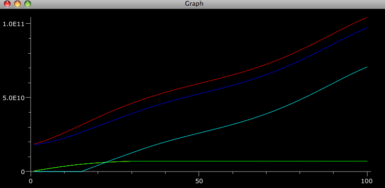
Figure 1: x-axis is years, y-axis is tonnes of CO2.
There is a catch, however; growth in emissions is both in the form of dispersed sources (cars, pastures, etc.) and point sources (power plants, etc.). All our alternative energies are electricity generation, and so cannot displace all emissions growth (in other words, building more nuclear power plants won't help cut growth in emissions from gasoline-fueled cars). At present, approximately half of all CO2 emissions come from point sources(Mahmoudkhani), not all of which are power generation.
This can be accounted for using a relatively simple trick. In the beginning, we will accomplish 40% of the reductions using alternative energies, and 60% using other emission reductions. With strict climate policy, the proportion of emissions is expected to shift significantly towards electrical sources (EPRI). Also note that our target of 350ppm is stricter than the scenarios presented in the EPRI report. Thus, as an estimate, we will assume that, by the end of the century, 75% of increase in emissions will be accounted for by alternatives, and 25% by renewables, and that there is a linear change in proportions. The graphs this results in are shown in [Figure 2]. RED are business as usual emissions, BLUE are net emissions,
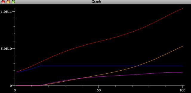
Figure 2: x-axis is years, y-axis is tonnes of CO2.
CAPABILITY 2: TRENDLINES
The program has four built-in trendlines - sigmoid, upper sigmoid, linear and exponential. The trendlines reflect how the CO2 reduction ability of each technology will increase over time. The section that follows is a rather technical explanation of how each curve equation is calculated. Note: for certain technologies (such as wind and natural gas), we created the trendline coordinates in excel and input them as a data file into the program for cost estimation (capability 3).
In order for the program to calculate any trendline, the following figures are essential:
1) xoffset = the year at which implementation of the technology begins
2) enddate = the year at which implementation should reach maximum capacity
3) uppertarget = the maximum rate of CO2 reduction, in tonnes, accomplished by the technology.
From this we define we timp, the time for implementation, as enddate - xoffset. Note that all trendlines are piecewise functions that assume y = 0 for all x < xoffset. For x >= xoffset and x <= enddate, the desired equation is used. For x > enddate, y = uppertarget
Sigmoid:
A sigmoid curve is characterised by a gradual rate of increase, followed by a period of very rapid implementaiton, followed by a gradual 'tapering off'
In addition to the aforementioned figures, the following two are necessary to make the sigmoid curve:
-> m = steepness constant (a constant that controls the steepness of the curve; the larger the steeper).
-> whereinflect = How many years after 'startdate' is the year of steepest implementation (point of inflection). Typically, half of timp (halfway through implementation) gives realistic curves.
The basic equation for a sigmoid curve is: y = 1/(1+e^-x). To get this to match the implementation curve, the following tranformations are applied:
1) Steepness is controlled by the factor multiplying x. A larger value of timp implies the curve should be less steep, since there is more time for implementation. However, the user should also be able to control steepness by varying m. Thus, the applied transformation is x --> (m/timp)*x
2) In the basic curve, the steepest implementation (point of inflection) is at t=0. The curve is thus translated forwards by whereinflect units (x --> x - whereinflect).
3) Translate the curve down so that y = 0 at x = 0. To do this, let yoffset be the value of the curve at x=0, and translate: (y --> y - yoffset).
4) Scale the curve up so that y = uppertarget at x = timp. To do this, let a be the value of y at x = timp, and s be uppertarget/a. Apply the stretch: (y --> s*y).
5) Translate the curve to the right by xoffset units. The translation is: (x --> x - xoffset).
Example: 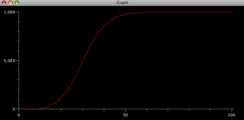
x-axis: years, y-axis: tonnes of CO2 reduction per year.
Input: xoffset = 10, enddate = 60, whereinflect = 20, uppertarget = 1000000, m = 9.
Upper Sigmoid:
The upper half of a sigmoid curve. This curve starts off at steepest implementation and gradually tapers away. The basic equation is: y = 1/(1+e^-x) - 0.5
The techniques are very similar to those used in a sigmoid curve. Since there is no point of inflection, the only required additional information is m, the steepness constant.
The following transformations are employed:
1) Introduce steepness, i.e: x --> (m/timp)*x
2) Scale the curve up so that y = uppertarget at x = timp.
3) Translate the curve to the right by xoffset units.
Example: 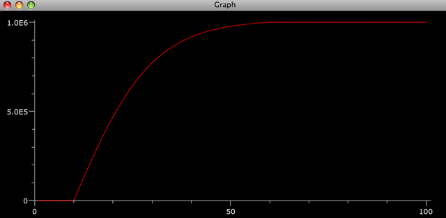
x-axis: years, y-axis: tonnes of CO2 reduction per year.
Input: xoffset = 10, enddate = 60, uppertarget = 1000000, m = 5.
Linear
This is the most basic of the curves. The gradient of the line is uppertarget/timp. The equation is: y = (uppertarget/timp)*(x - xoffset).
Exponential
This is an unrealistic curve because it involves an abrupt flattening at x = enddate. The only required added information is m, the steepness constant. The basic equation is y = e^x. The following transformations are used:
1) Shift the curve down by 1 unit so that y = 0 at x = 0.
2) Scale the curve up so that y = uppertarget at x = timp.
3) Translate the curve to the right by xoffset units.
CAPABILITY 3: COST MODELLING WITH LEARNING EFFECTS
The costs for any capture/sequestration technology fall under three basic categories. On a graph with 'CO2 captured per year in metric tonnes' on the y-axis and 'time in years' on the x-axis, they would be represented as described:
Variable cost: This is related to the amount of CO2 being captured. The annual expense is the height of the curve times the cost per metric ton of CO2.
Capital cost: This is related to the amount of new capital being added. The slope of the curve gives the increase in the rate of CO2 capture that year, and [slope]/[annual capture capacity per plant] gives the number of new plants built that year. Thus, annual capital cost = [cost per plant]*[slope]/[annual capture capacity per plant].
Operational and Maintenance costs: These depend on the number of plants that are operating in a given year. Since the number of plants is the height of the curve divided by the annual capture capacity per plant, annual operation/maintenance costs are: [operational/maintenance costs for one plant]*[height of curve]/[capture capacity per plant per year]
Learning Effects
Learning effects are characterized as follows: when the total past production doubles, the cost for producing subsequent units falls by a fixed percentage. For instance, if doubling past production decreases costs by 5%, then the cost of the nth unit is: A*(0.95)^[(log n)/(log 2)], where A is the initial cost of production.
A more sophisticated variation of this is when you take A to be the cost of the Pth unit. The cost of the nth unit then has to be found relative to the increase in production from P, and thus the cost is: A*(0.95)^[log(n/P)/(log 2)]. In the model, we took 'P' to be the production after one year.
The challenge, however, is how to quantify 'past production'. For the three categories mentioned, here is one possible approach:
- Variable cost: Total 'past CO2 captured' is the area under the curve
- Capital cost: Total plants built is the height of the curve divided by the capture per plant per year
- Operational/Maintenance cost: Total 'plant years' of operation/maintenance is the area under the curve divided by the capacity per plant per year.
Plugging the above values in place of 'n' would yield the costs for that particular category, adjusted for learning effects.
This learning effect was used to project a possible decrease in the price of air capture, assuming a 10% reduction with every doubling [Figure 5]. Note that this differs slightly from the values in the main graph elsewhere on the site because it account for a gradual build-up in the implementation of air capture.
(Cost without learning effect - 273 trillion. Cost with learning effect: 69.5
trillion).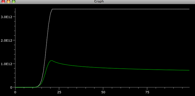
Figure 3: x-axis: years, y-axis: annual cost in dollars.
The total cost can then be found by doing a Riemann sum for the area under the curve.
An even more sophisticated approach would model a gradual trend in the learning effect over time. For the interest of the reader, a possible approach is described here. Let the 'b' value be (1 - %age decrease in cost), i.e., if costs reduce by 10% with every doubling, b = 0.9.
- Let the value of b change from b1 to b2 in the years t1 to t2. Thus, at a year t, the b value is b[t] = (b1 + (b2 - b1)*(t - t1)/(t2 - t1))
- Let the production at year t equal P[t]. Thus, the relative increase in production from year t-1 to year t is P[t]/P[t-1].
- Let C[t] denote the cost function. By the learning curve effect, the change in cost from year t-1 to year t is: C[t] = C[t-1]*(b[t])^{(log(P[t]/P[t-1])/log 2}
- Hence, given a starting cost, the costs in subsequent years can be found through iteration.
Note: for further details, including source code, feel free to contact: avanti.shrikumar {at} gmail {dot} com