Why 350?

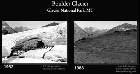
(USGS, 1988)

Boulder Glacier in 1932, and then again in 1988.

The fact that climate change is occurring is no longer in dispute among scientists. Figure 1 contains a graph of temperature trends of the Northern and Southern Hemispheres, juxtaposed to that of the entire Earth. The data is from measurements made by the Climatic Research Unit (CRU) of the University of East Anglia.

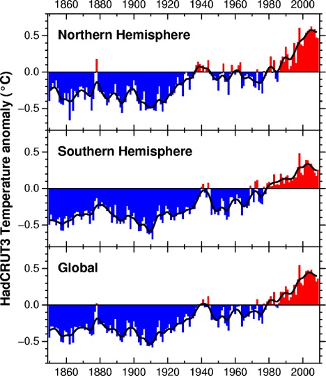
Figure 1 (Brohan, 2006)

As one can see, there has been a warming trend since 1980. Figure 2 shows the correlation between the global average surface temperature, the increase in sea level, and the decrease in surface albedo of the Northern Hemisphere.

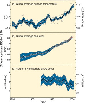
Figure 2 (IPCC Fourth Assessment Report: Climate Change, 2007)

There are many reasons to believe that an increase in temperature of 2°C or more would lead to irreversible global climate change. The real problem that climate scientists face today is ascertaining the effects of rapidly increasing anthropogenic carbon dioxide (CO₂) on our climate, and whether or not it would be feasible (or even desirable) to reduce its concentration in the atmosphere.

This 2° limit, with nominal climate sensitivity of approximately ¾ °C per W/m² and a reasonable control of other greenhouse gases (GHGs) would give a maximum concentration of CO₂ of approximately 450 parts per million . Using paleoclimate data (and the observable changes in the world’s climate) one can see that some “slow” feedback processes not included in most climate models, such as ice sheet disintegration, vegetation migration, and GHG release from soils, tundra, or ocean sediments (e.g. methane release from warming permafrost) may begin to have an effect within centuries. Tracking long-term climate changes reveals a high sensitivity to climate forcings such as a high CO₂ concentration. This knowledge, coupled with ongoing climate change, leaves us no choice but to reduce to less than the current level of CO₂. A goal of 350 ppm is recommended, but can be raised or lowered as models improve and knowledge of slow feedback mechanisms increases. (Hansen, 2008)

—Climate Sensitivity—

A global climate forcing, or radiative forcing, is a disturbance of the planet’s energy balance. Examples of forcings are increased greenhouse gas (GHG) concentrations, a change in solar luminosity (the brightness of the Sun), volcanic eruptions (a negative forcing), or a change in the earth’s orbit. Climate sensitivity is the temperature change per Watt per square meter of climate forcing.

Jule Charney, one of the founding fathers of meteorology, created an idealized scenario in which the global temperature change is measured after a doubling in atmospheric CO₂. The Charney estimate, though now considered outdated compared to more advanced models, is still a useful measure of comparison. The Charney estimate assumes that positive climate feedbacks that are considered “slow” such as ice sheets and forest cover remain constant. A positive feedback is a system in which an effect amplifies itself. For example, a warmer climate evaporates more water into the air, and since water vapor is a greenhouse gas, this causes more warming. This continues until equilibrium is reached. (Equilibrium occurs through a combination of carbon “sinks”, mostly the ocean. The concentrations of other long-lived GHGs are also assumed to remain relatively constant. What Charney does take into account is processes such as changes of water vapor, clouds, aerosols, and sea ice. Using only fast feedbacks, the Charney estimate was calculated to be 3±1.5°C. (Hansen, 2008)

—Pleistocene Epoch—

The atmospheric composition and surface properties of the late Pleistocene are known well enough to assess the accuracy of the Charney climate sensitivity. Since an imbalance of even 1 W/m² held over a few thousand years would either melt all ice on the planet or lead to a dramatic change in ocean temperature, the planet must necessarily have been in energy balance within a fraction of 1 W/m² in both the pre-Industrial Holocene period and the last glacial maximum (LGM), or ice age, which took place about 20ky BP (20,000 years before present). The difference now is that GHGs are rising at a rate faster than the climate system can respond. (Hansen, 2008)

The total climate forcing in the LGM equilibrium is about 6.5 W/m² relative to the Holocene period, corresponding to a global temperature change of 5±1°C. This is the sum of two different climate forcings. The different global surface properties of the ice age are the first. The increased ice area, different distribution of vegetation, and increased exposure of continental shelves contributed -3.5±1 W/m². The reduced amount of long-lived GHGs such as CO₂, nitrous oxide (N₂O), and methane (CH₄) is the second. This contributed -3±0.5 W/m². Forcing due to slight changes in the earth’s orbit is negligible (a small fraction of 1 W/m²). Calculations using this data would yield an empirical climate sensitivity of approximately¾ °C per W/m², or a Charney sensitivity of 3±1.5°C. (Hansen, 2008)

The climate sensitivity does not remain constant; rather, it varies with global temperature due to positive feedback systems. As the Earth grows colder, the surface area of sea ice grows, increasing the albedo effect. Albedo is the fraction of solar radiation reflected from a surface. (The ice caps, for example, have a very high albedo.) The increase of high-albedo surfaces increases the total amount of radiation re-radiated into the atmosphere, thus cooling the Earth even further. This is a positive feedback, as more cooling will again increase albedo feedback, and so on. The cycle, left unmitigated, can cause the Earth to eventually enter an ice age. At high temperatures the reverse can happen, and the Earth hits a runaway greenhouse effect. Eventually, equilibrium will be reached. This is a combination of the ocean, soil, vegetation, and weathering. Weathering involves the breakdown of minerals through chemical interactions with the atmosphere. CO₂ reacts with water to break down limestone (CaCO₃). Negative feedbacks such as the weathering of minerals, however, takes place on much longer time scales, and cannot be counted on to solve our current problem. (IPCC, 2007 and Hansen, 2008)

Currently, we are in a relatively stable interglacial period, which means that we are between ice ages. This also means that we are on a flat portion of our fast-feedback climate sensitivity curve. Therefore the calculated fast-feedback climate sensitivity, although simply a mean between the ice age and our interglacial period, is very close to the fast-feedback climate sensitivity of today. (Hansen, 2008)

This sensitivity can be checked against a longer, continuous period of time using data from the Antarctic Vostok ice core showing CO₂ and CH₄ concentrations, as well as data from Red Sea sediment cores showing sea level changes. Gas concentrations in Figure (2a) are from the same ice core and consistent with the timeline, but sea level dating has an error bar on the order of several thousand years.

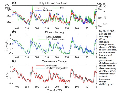
Figure 3 (Hansen, 2008)

Figure (3b) is a graph of climate forcing over time. The blue curve is calculated by multiplying the total GHG and surface albedo forcings by the fast-feedback climate sensitivity. The Antarctic temperature change divided by two (red curve in Figure (3c)) is a crude approximation of global temperature change. (The typical mean global temperature change is between glacial periods is approximately 5°C, with a 10°C change in the Antarctic.) The calculated temperature and observed temperature curves are relatively consistent. (Hansen, 2008)

Over thousands of years, slower feedback systems come into play. Over such long periods of time one can assume that the earth remains in relative energy balance, with the ocean’s slow thermal response time minimized, and the changes in temperature global. Examples of “slow” feedbacks include ice sheet disintegration, vegetation migration, and GHG release from soil, permafrost, and the ocean. The greatest increase in GHG concentrations is due to the release of CO₂ by the oceans. For one, CO₂ solubility decreases as temperature increases. Additionally, there is increased ocean mixing in a warmer climate, where cooler and deeper water replaces warmer water nearer the surface. This increased mixing of water helps to move carbon dioxide normally trapped deep in the ocean to the surface, where it evaporates into the atmosphere. These feedbacks have a very powerful effect on the climate. However, they do not typically initiate these changes. This is evidenced by the fact that changes in GHG concentrations and sea levels (an indirect measure of ice cap size) lag changes in temperature by several hundred years. Rather, it is the sure and slow change of the Earth’s orbit, specifically the tilt of the rotational axis, which begins the large glacial-interglacial climate changes. The forcing due to this change is comparatively small, but effect of the orbital change on the ice sheets can be large. For example, when the spin-axis tilt increases, ice melts at both poles. This decreases surface albedo, which acts as a positive feedback to produce more warming, and thus amplify ice sheet disintegration and GHG release. (Hansen, 2008)

The climate sensitivity on the longer Pleistocene time scales includes the effects of these slow feedbacks, and because the largest feedbacks are positive, it is greater than the Charney sensitivity. Use of this paleoclimate data allows scientists to calculate the long-term climate sensitivity. Figure 4 gives a graph of GHG forcing data from ice cores as a function of temperature, yielding a climate sensitivity of 1.5°C per W/m². (Hansen, 2008)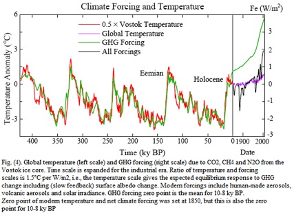

Figure 4 (Hansen, 2008)

The time to reach thermal equilibrium depends on many factors. For one, carbon dioxide does not disappear from the atmosphere nearly as quickly as other GHGs. As CO₂ emissions increase, the carbon-buffer chemistry of the ocean decreases, meaning that the ocean becomes saturated with CO₂. In addition, although the terrestrial biosphere does absorb CO₂ at a nearly constant rate, this too may become saturated within decades, leaving the already-strained ocean-atmosphere system to absorb the additional CO₂. (Archer, 2009)

It is important to delineate the amount of time it takes the ocean-atmosphere and ice sheet-atmosphere systems to respond to a changing climate. The ocean-caused delay depends very strongly upon the climate sensitivity. In fact it varies almost quadratically, with half of the response occurring in only a few years, three quarters in 250 years, and the rest taking at least a thousand years. Ice sheet response is difficult to model, due to gaps in knowledge of the physics of ice sheet disintegration. Crude models typically make use of paleo sea level data that captures the broad range of sea level change. However, this data may simply be modeling the small, slow forcing of the Earth’s orbital changes, and glossing over very important data. Higher time-resolution paleo sea level data reveal changes as great as 1m per century, information that is lost when averaging climate over much longer periods of time. In addition, this was due to forcings weaker than the anthropogenic forcing now. Therefore it is probable that ice sheet disintegration will occur within several hundred years on a large scale unless the forcing is soon reduced. Changes in sea level may become substantial. (Hansen, 2008)

—Cenozoic Era—

Normally when we think of the CO₂ feedback systems, we think of the exchange of CO₂ between the ocean and atmosphere. This is generally the most important. But on much longer time scales, weathering becomes significant.

The Cenozoic era reaches back to the past 65.5 million years. Even though data is not as precise, it is useful to compare atmospheric and climate conditions between these larger climate variations.

The temperature decrease between the ice-free period 50 mya and the ice age 20 kya was approximately 14°C, a forcing due entirely to changes in the atmosphere. The only other forces possible would have been due to changes in solar irradiance or due to shifts in continental locations. However, solar brightness actually increased in that time by a small amount (0.4%, corresponding to 1W/m²) and continents were already close to present locations. The CO₂ concentrations, on the other hand, differ from about 180 ppm during the ice age and 1500±500 ppm in the early ice-free Cenozoic. This is a forcing of roughly 10W/m², enough to account for the difference in temperatures. Approximately 35 mya Antarctica began to glaciate (i.e. freeze over). This point is used because between 65 and 35 mya, the feedbacks in play were mostly fast, making it easier to model. Also, it is important to know the temperature at which Antarctic glaciation occurred. Since glaciation is reversible, this number can then be compared to new data on CO₂ amount. Using climate models and knowledge of the forcing, one can simulate what would happen if the concentration of CO₂ were given a specific value at 35 mya. If the resulting curve matches well with actual data, then that initial concentration was a correct assumption. At the point when Antarctica glaciated, a CO₂ concentration of about450±100 ppm fits well. Given what we know of forcing and feedback systems, this implies that the Charney climate sensitivity is not valid when predicting the equilibrium temperature at doubled CO₂ concentrations. There is additional warming due to slow feedbacks such as ice loss and the spread of vegetation, almost doubling the equilibrium climate sensitivity. With doubled CO₂ it would take many decades for the majority of equilibrium to be reached because of the long ocean and ice sheet thermal response times. But looking at Earth’s geologic history, it can be seen that positive feedbacks such as a reduction in sea ice area (and the surface albedo effect) can cause relatively large warming trends, with large fluctuations in sea level. If humans were to force the Earth’s climate sufficiently, then positive feedback systems would take over and it would be impossible to prevent them. (Hansen, 2008)

—Anthropocene Era—

The Anthropocene era began 6 to 8 thousand years ago. Prior to the Industrial Revolution, forcing due to anthropogenic CO₂ was very small, or possibly negative. However, increased fossil fuel use in the past twenty-five years has created a forcing large enough to overpower any negative forcings.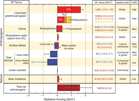

Figure 5 (IPCC Fourth Assessment Report: Climate Change, 2007)

There are two highly important levels of forcing. One is the tipping level, or “the global climate forcing that, if long maintained, gives rise to a specific consequence,” and two is the “point of no return, a climate state beyond which the consequence is inevitable, even if climate forcings are reduced.” One can exceed the tipping level and still be able to decrease in time to prevent any significant climate change. The magnitude and length of time that one can exceed this level is difficult to ascertain, but if it has been maintained for a long enough time, re-equilibration will not occur without some severe consequences. Once the point of no return is reached negative climate effects continue to occur no matter how much the atmospheric CO₂ is reduced, as positive feedbacks will have taken over. (Hansen, 2008)

It is difficult to infer a point of no return due to model inaccuracies and the nature of the data. On the other hand, tipping levels are easier to pinpoint, partially because of the fact that the magnitude and time allowance are undefined. One can estimate it through analysis of the climate swings of Earth’s past.

—Target—

Although positive anthropogenic forcing of other GHGs (N₂O, CH₄) exists, the amount now being emitted is lower than what the IPCC has predicted. Aerosols are a negative forcing and have a cooling effect on the planet. Therefore, these raise the maximum allowable GHG emissions. The use of aerosols, along with the fact that lower amounts of other GHGs are being emitted, means that the effects of non-CO₂ GHGs are almost neutralized. This leaves CO₂ concentrations as the major source of forcing for any climate change. Considering the Cenozoic era, the point at which Antarctica glaciates (and hence also the point at which it would melt) was estimated to be 450 ppm. A target concentration would therefore have to be lower to prevent large-scale climate change. The current changes in climate suggest that 387 ppm is already too high. (See Negative Effects of Climate Change ) Current models show that there is currently a +0.5-1 W/m² energy imbalance and this estimate is supported by the temperature increase in the upper 700m of the ocean. However, the change in temperature over the entire volume of the oceans must be measured to properly quantify this estimate. Yet given what we do know, a reduction to 300-350 ppm would be needed to prevent further ice cap loss and ocean acidification. (Hansen, 2008)

—Uncertainties—

The climate is an extremely complex system, and many variables which affect climate are difficult to model realistically. For example, knowledge of the way in which aerosols equilibrate, or ice sheets disintegrate, is limited. Natural variability could thus account for much of the changes in temperature. However, knowledge of some of the causes of natural variability, as well as climate forcing models, rules out its being the sole cause, and gives a reasonable error bar. These uncertainties can both overestimate or underestimate the effects of anthropogenic forcing. In other words, the models may be giving a very conservative view of the effects of anthropogenic emissions.

—Conclusion—

Slow feedbacks have been shown to be relevant to an analysis of target CO₂ concentrations, as they nearly double the Charney climate sensitivity. This doubled sensitivity means that atmospheric concentrations of GHGs originally thought safe would, maintained over a long enough period of time, actually lead to serious irreversible climate change. Ice sheet collapse, the migration of plants cover in the Northern Hemisphere, and the release of GHGs from frozen tundra and soil are all slower feedbacks which would eventually come into play. Essentially, the problem is determining the tipping level at which this occurs, and the amount of time we can safely exceed it. A tentative estimate using paleoclimate data, and taking into account the changes in climate already occurring, is 350 ppm. This number will have to be readjusted as knowledge of climate systems and observed trends changes, but serves as a boundary to atmospheric concentrations to work towards.